Investment Portfolio Optimization
Originally Posted: December 04, 2015
The need to make trade-offs between the effort exerted on specific activities is felt universally by individuals, organizations, and nations. In many cases, activities are mutally-exclusive so partaking in one option excludes participation in another. Deciding how to make these trade-offs can be immensely difficult, especially when we lack quantitative data about risk and reward to support our decision.
In the case of financial assets, there is a wealth of numerical data available. So in this post, I explore how historical data can be leveraged to choose specific mixes of assets based on investment goals. The tools used are quite simple and rely on the mean-variance of assets’ returns to find the efficient frontier of a portfolio.
Note: The code and data used to generate the plots in this post are available here.
Historical Stock Price Data
Most people have probably interacted with Google Finance or Yahoo! Finance to access financial information about stocks. The Python library Pandas provides an exceedingly simple interface for pulling stock quotes from either of these sources:
#Import Pandas web data access library
import pandas.io.data as web

#Request quote information for Tesla's stock denoted by the symbol 'TSLA'
tslaQuote = web.DataReader('TSLA', data_source='yahoo', start='2010-01-01',
                           end='2014-12-31')
This integration makes pulling historical pice data very easy, which is great since we want to estimate portfolio performance using past pricing data.
Basic Portfolio Theory
Investopedia defines “Portfolio theory” as:
Modern Portfolio Theory - MPT A theory on how risk-averse investors can construct portfolios to optimize or maximize expected return based on a given level of market risk, emphasizing that risk is an inherent part of higher reward. “Modern Portfolio Theory - MPT.” Investopedia.com. Investopedia, 2015. Web. 5 December 2015.
The idea is the fundamental concept of diversification and essentially boils down to the idea that pooling risky assets together, such that the combined expected return is aligned with an investor’s target, will provide a lower risk-level than carrying just one or two assets by themselves. The technique is even more effective when the assets are not well correlated with one another.
Portfolio theory’s efficacy can be seen by examining the underlying statistical thoughts behind the concept. For a single asset, the expected mean-variance of returns ‘r’ over ‘n’ observations is given by the standard formulas below.
\[\begin{align*} & Mean(Returns) = \frac{1}{n} \sum_{i=1}^{n}r_i \\ & Var(Returns) = \sum_{i=1}^{n}(r_i-\mu)^2 \\ \end{align*}\]Expanding this to the mean-variance of a portfolio of assets that are potentially correlated to one another, we have the weighted average of the mean returns, and the sum of the terms in the covariance matrix for the assets:
\[\begin{align*} & Mean(Portfolio\ Returns) = \sum_{i=1}^{n}w_i r_i \\ & Var(Portfolio\ Returns) = \sum_{i=1}^{n}\sum_{j=1}^{n}w_i w_j \rho_{i,j} \sigma_i \sigma_j = \mathbf{w}^T \bullet \big(\mathbf{cov} \bullet \mathbf{w}\big) \\ \end{align*}\]The Python package NumPy provides us with all of the functions necessary to calculate the mean-variance of returns for individual assets and portfolios, including vector math operations to keep the code clean.
#Set the stock symbols, data source, and time range
stocks = ['GOOGL', 'TM', 'KO', 'PEP']
numAssets = len(stocks)
source = 'yahoo'
start = '2010-01-01'
end = '2015-10-31'

#Retrieve stock price data and save just the dividend adjusted closing prices
for symbol in stocks:
        data[symbol] = web.DataReader(symbol, data_source=source, start=start, end=end)['Adj Close']

#Calculate simple linear returns
returns = (data - data.shift(1)) / data.shift(1)

#Calculate individual mean returns and covariance between the stocks
meanDailyReturns = returns.mean()
covMatrix = returns.cov()

#Calculate expected portfolio performance
weights = [0.5, 0.2, 0.2, 0.1]
portReturn = np.sum( meanDailyReturns*weights )
portStdDev = np.sqrt(np.dot(weights.T, np.dot(covMatrix, weights)))
This is great, if we have a set of assets and their weights within a portfolio, abut 20 lines of Python will retrieve historical quotes, calculate the mean-variance of the assets, and return the expected portfolio performance. But what if we didn’t know which assets to purchase and in what proportion to one another? Surely there are multiple ways to achieve a target return and perhaps those different asset blends will yield varying amounts of risk while providing the same return.
Monte Carlo Method
One approach to optimizing a portfolio is application of the Monte Carlo Method. For unfamiliar readers, this is the idea of carrying out repeated trials using randomly generated inputs and observing the outcomes. A physical example of this would be flipping a coin 100 times and counting the number of heads and tails. Based on the results, the observer could estimate whether the coin is fair or not. In the digital world, computers can rapid generate random numbers extremely quickly, enabling observation of outcomes from complex scenarios that are based on the probabilities of certain events occurring. The code below illustrates how simple it is to implement a Monte Carlo simulation using Python:
#Run MC simulation of numPortfolios portfolios
numPortfolios = 25000
results = np.zeros((3,numPortfolios))

#Calculate portfolios
for i in range(numPortfolios):
    #Draw numAssets random numbers and normalize them to be the portfolio weights
    weights = np.random.random(numAssets)
    weights /= np.sum(weights)

    #Calculate expected return and volatility of portfolio
    pret, pvar = calcPortfolioPerf(weights, meanDailyReturn, covariance)

    #Convert results to annual basis, calculate Sharpe Ratio, and store them
    results[0,i] = pret*numPeriodsAnnually
    results[1,i] = pvar*np.sqrt(numPeriodsAnnually)
    results[2,i] = (results[0,i] - riskFreeRate)/results[1,i]
In the plot below, 25,000 portfolios with randomly varying weights of the following assets were generated and evaluated. Their expected annual return is then plotted versus the historical volatility of the portfolio. Further, each point representing a portfolio has been shaded according to the “Sharpe Ratio.”
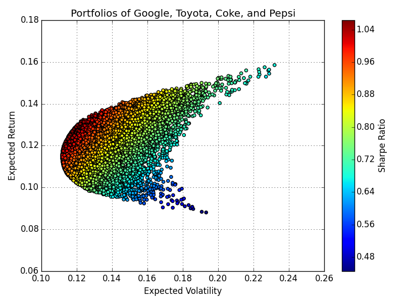
From Figure 1 it is obvious that changing the weight of each asset in the portfolio will have a dramatic effect on the expected return and the level of risk that the investor is exposed to. Most notably, if the investor is targeting a 12% return it is evident that the volatility could be reduced to 11.5% but some portfolios share that same expected return with as high as 17.5% volatility. Figure 1 makes it very clear that we must be thoughtful when choosing how much weight each asset in our portfolio should carry.
Efficient Frontier and Portfolio Optimization
Based on the insights from Figure 1, it is evident that a target return can be achieved with a wide range of risk levels. This introduces the concept of the “Efficient Frontier.” The Efficient Frontier is the set of portfolios that achieve a given return with the minimum amount of risk for that return. In Figure 1, these were the portfolios furthest to the left for each expected return.
Keeping this concept in mind, a more structured approach can be applied to the selection of asset weights such that we consider only these efficient portfolios which meet a criteria important to the investor. First, she could optimize the weights to target a metric such as the Sharpe Ratio. Alternatively, the investor could opt to find the minimum volatility portfolio and accept the return that that provides. The code below consists of several helper functions that make use of SciPy’s optimization library to solve these two problems.
import numpy as np
import scipy.optimize as sco

def calcPortfolioPerf(weights, meanReturns, covMatrix):
    '''
    Calculates the expected mean of returns and volatility for a portolio of
    assets, each carrying the weight specified by weights

    INPUT
    weights: array specifying the weight of each asset in the portfolio
    meanReturns: mean values of each asset's returns
    covMatrix: covariance of each asset in the portfolio

    OUTPUT
    tuple containing the portfolio return and volatility
    '''
    #Calculate return and variance
    portReturn = np.sum( meanReturns*weights )
    portStdDev = np.sqrt(np.dot(weights.T, np.dot(covMatrix, weights)))

    return portReturn, portStdDev

def negSharpeRatio(weights, meanReturns, covMatrix, riskFreeRate):
    '''
    Returns the negated Sharpe Ratio for the speicified portfolio of assets

    INPUT
    weights: array specifying the weight of each asset in the portfolio
    meanReturns: mean values of each asset's returns
    covMatrix: covariance of each asset in the portfolio
    riskFreeRate: time value of money
    '''
    p_ret, p_var = calcPortfolioPerf(weights, meanReturns, covMatrix)

    return -(p_ret - riskFreeRate) / p_var

def getPortfolioVol(weights, meanReturns, covMatrix):
    '''
    Returns the volatility of the specified portfolio of assets

    INPUT
    weights: array specifying the weight of each asset in the portfolio
    meanReturns: mean values of each asset's returns
    covMatrix: covariance of each asset in the portfolio

    OUTPUT
    The portfolio's volatility
    '''
    return calcPortfolioPerf(weights, meanReturns, covMatrix)[1]

def findMaxSharpeRatioPortfolio(meanReturns, covMatrix, riskFreeRate):
    '''
    Finds the portfolio of assets providing the maximum Sharpe Ratio

    INPUT
    meanReturns: mean values of each asset's returns
    covMatrix: covariance of each asset in the portfolio
    riskFreeRate: time value of money
    '''
    numAssets = len(meanReturns)
    args = (meanReturns, covMatrix, riskFreeRate)
    constraints = ({'type': 'eq', 'fun': lambda x: np.sum(x) - 1})
    bounds = tuple( (0,1) for asset in range(numAssets))

    opts = sco.minimize(negSharpeRatio, numAssets*[1./numAssets,], args=args,
                        method='SLSQP', bounds=bounds, constraints=constraints)

    return opts

def findMinVariancePortfolio(meanReturns, covMatrix):
    '''
    Finds the portfolio of assets providing the lowest volatility

    INPUT
    meanReturns: mean values of each asset's returns
    covMatrix: covariance of each asset in the portfolio
    '''
    numAssets = len(meanReturns)
    args = (meanReturns, covMatrix)
    constraints = ({'type': 'eq', 'fun': lambda x: np.sum(x) - 1})
    bounds = tuple( (0,1) for asset in range(numAssets))

    opts = sco.minimize(getPortfolioVol, numAssets*[1./numAssets,], args=args,
                        method='SLSQP', bounds=bounds, constraints=constraints)

    return opts

#Find portfolio with maximum Sharpe ratio
maxSharpe = findMaxSharpeRatioPortfolio(weights, meanDailyReturn, covariance,
                                        riskFreeRate)
rp, sdp = calcPortfolioPerf(maxSharpe['x'], meanDailyReturn, covariance)

#Find portfolio with minimum variance
minVar = findMinVariancePortfolio(weights, meanDailyReturn, covariance)
rp, sdp = calcPortfolioPerf(minVar['x'], meanDailyReturn, covariance)
Figure 2 shows results from these optimizations, the portfolios with the highest Sharpe Ratio and lowest volatility are denoted by the red and yellow stars respectively.
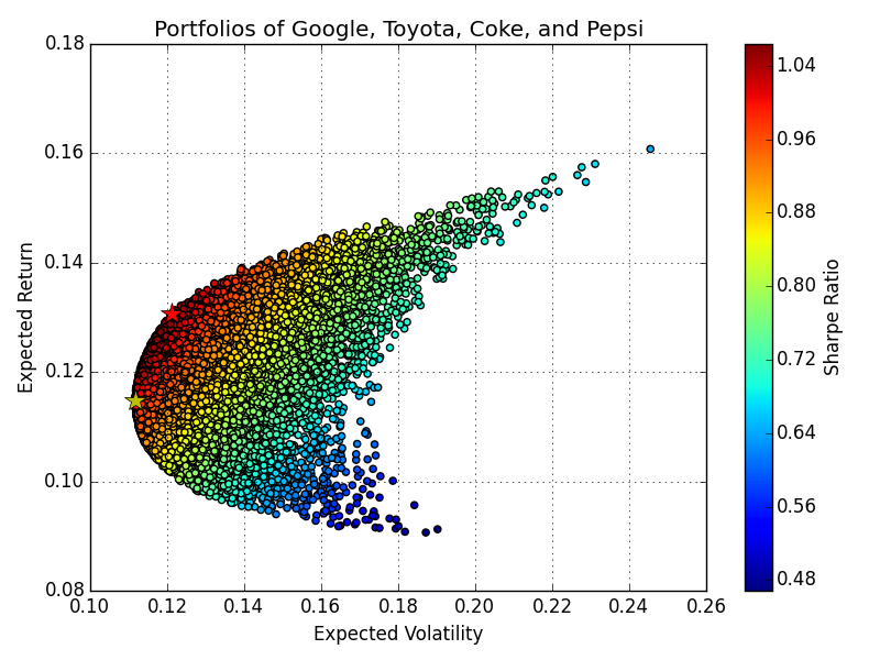
This structured approach can be taken a step further to find the Efficient Frontier across a range of desired target returns. The set of portfolios that provide a target return with minimum volatility is found by iteratively applying the SciPy optimizer as shown in the code below. Figure 3 shows the results for this optimization.
def findEfficientReturn(meanReturns, covMatrix, targetReturn):
    '''
    Finds the portfolio of assets providing the target return with lowest
    volatility

    INPUT
    meanReturns: mean values of each asset's returns
    covMatrix: covariance of each asset in the portfolio
    targetReturn: APR of target expected return

    OUTPUT
    Dictionary of results from optimization
    '''
    numAssets = len(meanReturns)
    args = (meanReturns, covMatrix)

    def getPortfolioReturn(weights):
        return calcPortfolioPerf(weights, meanReturns, covMatrix)[0]

    constraints = ({'type': 'eq', 'fun': lambda x: getPortfolioReturn(x) - targetReturn},
                   {'type': 'eq', 'fun': lambda x: np.sum(x) - 1})
    bounds = tuple((0,1) for asset in range(numAssets))

    return sco.minimize(getPortfolioVol, numAssets*[1./numAssets,], args=args, method='SLSQP', bounds=bounds, constraints=constraints)

def findEfficientFrontier(meanReturns, covMatrix, rangeOfReturns):
    '''
    Finds the set of portfolios comprising the efficient frontier

    INPUT
    meanReturns: mean values of each asset's returns
    covMatrix: covariance of each asset in the portfolio
    targetReturn: APR of target expected return

    OUTPUT
    Dictionary of results from optimization
    '''
    efficientPortfolios = []
    for ret in rangeOfReturns:
        efficientPortfolios.append(findEfficientReturn(meanReturns, covMatrix, ret))

    return efficientPortfolios

#Find efficient frontier, annual target returns of 9% and 16% are converted to
#match period of mean returns calculated previously
targetReturns = np.linspace(0.09, 0.16, 50)/(252./dur)
efficientPortfolios = findEfficientFrontier(meanDailyReturn, covariance, targetReturns)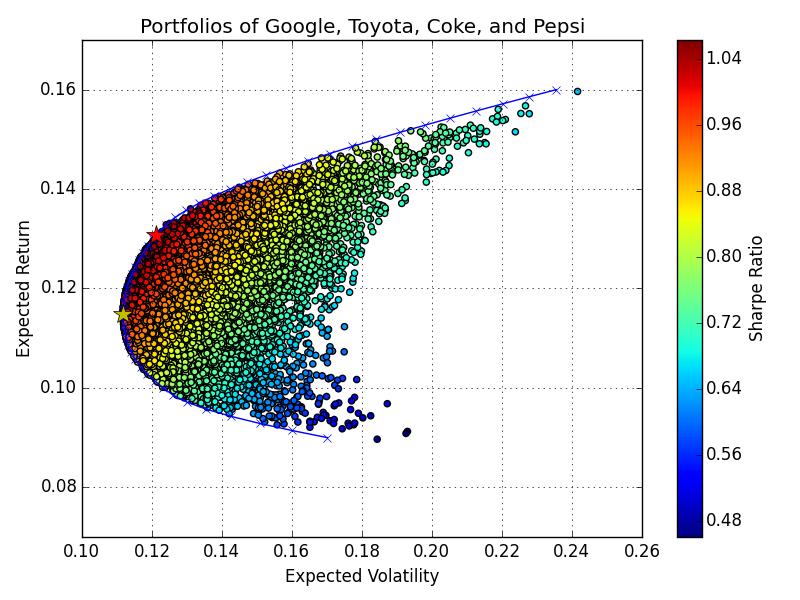
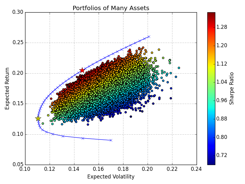
Optimum Portfolio of Many Assets
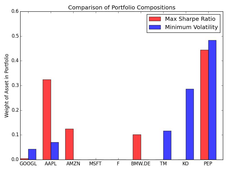
The framework developed up to the point can readily be applied to find the optimum portfolio when an investor is faced with choosing from many assets. Figure 4 below shows the results for a portfolio consisting of Apple, Amazon, BMW, Coke, Ford, Google, Microsoft, Pepsi, and Toyota. Figure 5 shows the weights of each asset for the Sharpe Ratio maximizing and minimum volatility portfolios.