Assessing Credit Risk with the Merton Distance to Default Model

Originally Posted: May 20, 2017

One of the most effective methods for rating credit risk is built on the Merton Distance to Default model, also known as simply the Merton Model. While implementing this for some research, I was disappointed by the amount of information and formal implementations of the model readily available on the internet given how ubiquitous the model is. This post walks through the model and an implementation in Python that makes use of Numpy and Scipy.

The Merton Model

The Merton KMV model attempts to estimate probability of default by comparing a firm’s value to the face value of its debt. Since the market value of a levered firm isn’t observable, the Merton model attempts to infer it from the market value of the firm’s equity. If the firm’s debt is treated as a single zero-coupon bond with maturity T, then the firm’s equity becomes a call option on the firm value with a strike price equal to the firm’s debt. As an example, consider a firm at maturity: if the firm value is below the face value of the firm’s debt then the equity holders will walk away and let the firm default. But if the firm value exceeds the face value of the debt, then the equity holders would want to exercise the option and collect the difference between the firm value and the debt.

Inferring Firm Value

More formally, the equity value can be represented by the Black-Scholes option pricing equation. When the volatility of equity is considered constant within the time period T, the equity value is:

where V is the firm value, t is the duration, E is the equity value as a function of firm value and time duration, r is the risk-free rate for the duration T, \(\mathcal{N}\) is the cumulative normal distribution, and \(d_1\) and \(d_2\) are defined as:

Additionally, from Ito’s Lemma (Which is essentially the chain rule but for stochastic diff equations), we have that:

Finally, in the B-S equation, it can be shown that \(\frac{\partial E}{\partial V}\) is \(\mathcal{N}(d_1)\) thus the volatility of equity is:

Coding It Up

At this point, Scipy could simultaneously solve for the asset value and volatility given our equations above for the equity value and volatility. But, Crosbie and Bohn (2003) state that a simultaneous solution for these equations yields poor results. Instead, they suggest using an inner and outer loop technique to solve for asset value and volatility.

The inner loop solves for the firm value, V, for a daily time history of equity values assuming a fixed asset volatility, \(\sigma_a\). The outer loop then recalculates \(\sigma_a\) based on the updated asset values, V. Then this process is repeated until \(\sigma_a\) converges.

For the inner loop, Scipy’s root solver is used to solve:

This equation is wrapped in a Python function which accepts the firm asset value as an input:

def equations(v_a, debug=False):
    d1 = (np.log(v_a/face_val_debt) + (r_f + 0.5*sigma_a**2)*T)/(sigma_a*np.sqrt(T))
    d2 = d1 - sigma_a*np.sqrt(T)

    y1 = v_e - (v_a*norm.cdf(d1) - np.exp(-r_f*T)*face_val_debt*norm.cdf(d2))

    if debug:
        print("d1 = {:.6f}".format(d1))
        print("d2 = {:.6f}".format(d2))
        print("Error = {:.6f}".format(y1))

    return y1

Given this set of asset values, an updated asset volatility is computed and compared to the previous value. If it is within the convergence tolerance, then the loop exits. In Python, we have:

# Update sigma_a based on new values of Va
# First, save previous value of sigma_a
last_sigma_a = sigma_a

# Slice results for past year (252 trading days)
v_a_per = results[t-252:t,i]

# Calculate log returns
v_a_ret = np.log(v_a_per/np.roll(v_a_per,1))
v_a_ret[0] = np.nan

# Calculate new asset volatility
sigma_a = np.nanstd(v_a_ret)

if abs(last_sigma_a - sigma_a) < 1e-3:
  break

The full implementation is available here under the function solve_for_asset_value.

Getting to Probability of Default

Given the output from solve_for_asset_value, it is possible to calculate a firm’s probability of default according to the Merton Distance to Default model. The first step is calculating Distance to Default:

Where the risk-free rate has been replaced with the expected firm asset drift, \(\mu\), which is typically estimated from a company’s peer group of similar firms.

If we assume that the expected frequency of default follows a normal distribution (which is not the best assumption if we want to calculate the true probability of default, but may suffice for simply rank ordering firms by credit worthiness), then the probability of default is given by:

Some Results

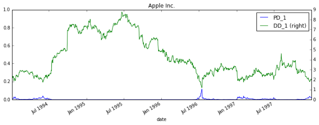
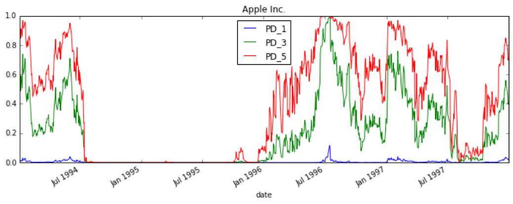
Below are the results for Distance to Default and Probability of Default from applying the model to Apple in the mid 1990’s. During this time, Apple was struggling but ultimately did not default. The model quantifies this, providing a default probability of ~15% over a one year time horizon.

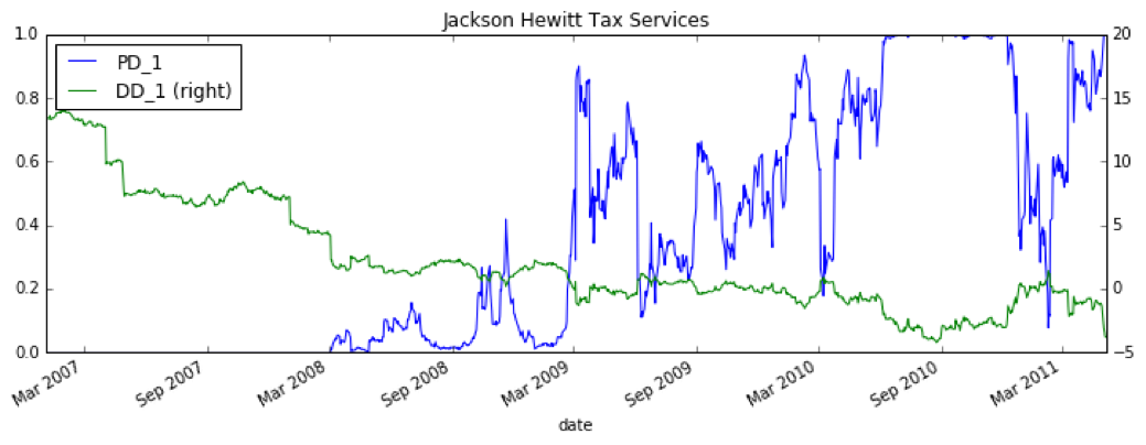
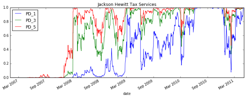
Results for Jackson Hewitt Tax Services, which ultimately defaulted in August 2011, show a significantly higher probability of default over the one year time horizon leading up to their default:

Conclusion

The Merton Distance to Default model is fairly straightforward to implement in Python using Scipy and Numpy. The results are quite interesting given their ability to incorporate public market opinions into a default forecast. That said, the final step of translating Distance to Default into Probability of Default using a normal distribution is unrealistic since the actual distribution likely has much fatter tails. It would be interesting to develop a more accurate transfer function using a database of defaults.